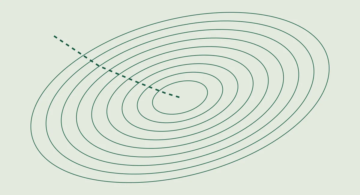
Optimization often begins with a simple question: which direction makes an error smaller? Gradient descent turns that local question into a repeatable procedure.
Start with a landscape
For a differentiable objective , the gradient points in the direction of steepest local increase in Euclidean space. A small step in the opposite direction is a useful first approximation to improvement.
Here is the learning rate. Choosing it is part of the algorithm, not an incidental implementation detail.
A minimal implementation
For , the derivative is . Start at and take ten steps:
def minimize(x: float, rate: float, steps: int) -> float:
    for _ in range(steps):
        gradient = 2 * x
        x -= rate * gradient
    return x

print(minimize(x=4.0, rate=0.2, steps=10))
# Approximately 0.0242
This is intentionally small enough to inspect by hand. Every iteration multiplies by . Convergence therefore requires , or .
Explore the learning rate
The control below computes one step for the same quadratic. At the largest rate it oscillates rather than improving.
| Learning rate | First step | Behavior for this quadratic |
|---|---|---|
| 0.1 | 3.2 | Gradual convergence |
| 0.5 | 0.0 | Reaches the minimum |
| 1.0 | -4.0 | Oscillation |
Know the assumptions
A useful algorithm can still fail when its assumptions change. Nonconvex losses have saddle points; noisy gradients change the trajectory; poorly scaled coordinates slow progress.
Measure the objective as well as the parameter update. A moving parameter is not evidence of a better model.
Further reading
Boyd and Vandenberghe’s Convex Optimization develops the mathematical background.1 For an infrastructure perspective, read the static publishing example.
Footnotes
-
Stephen Boyd and Lieven Vandenberghe, Convex Optimization, Cambridge University Press, 2004. See the freely available book on the authors’ website. ↩
Discussion
Comments are not enabled yet. Thank you for reading.